


TEC Measurement Method Based on Space-based AIS Data
-
摘要: 基于星载船舶自动识别系统(AIS),提出一种计算全球电离层电子总含量(TEC)的方法。通过在卫星上搭载两个相互垂直的线极化天线,测量AIS信号穿过电离层时的法拉第旋转角,再通过法拉第旋转角与TEC的关系估算TEC。基于天拓五号卫星的AIS数据进行了实验验证,并分析了硬件设备误差和观测参数误差对结果造成的影响。实验表明,本方法测量出的TEC值与基于全球定位系统(GPS)测量的TEC值差值平均为0.762 TECU,证明了此方法的可行性。与现有的TEC测量方法相比,该方法只需利用现有的AIS系统,无需部署地面站,可大幅提高数据更新速率。Abstract: A method to calculate the Total Electron Content (TEC) of the global ionosphere is proposed based on the Automatic Identification System (AIS) for ships on board. Specifically, The Faraday rotation angle of AIS signal passing through the ionosphere is measured by carrying two mutually perpendicular linearly polarized antennas on the satellite, and then estimate TEC by the relationship between the Faraday rotation angle and the TEC. The experimental validation based on the AIS data from Tiantuo V satellite is carried out, and the effects of hardware equipment errors and observation parameter errors on the results are analyzed. Experiments show that the difference between the TEC value measured by the method and by the Global Positioning System (GPS) is 0.762 TECU on average, which proves the feasibility of this method. Compared with the existing TEC measurement methods, this method only needs to use the existing AIS system without deploying ground stations, which can significantly improve the data update rate.
-
Key words:
- Space-based AIS /
- Faraday rotation angle /
- TEC /
- Satellite
-

图 1 用于TEC测量的星载AIS系统
Figure 1. Schematic diagram of the space-based AIS system for TEC measurement

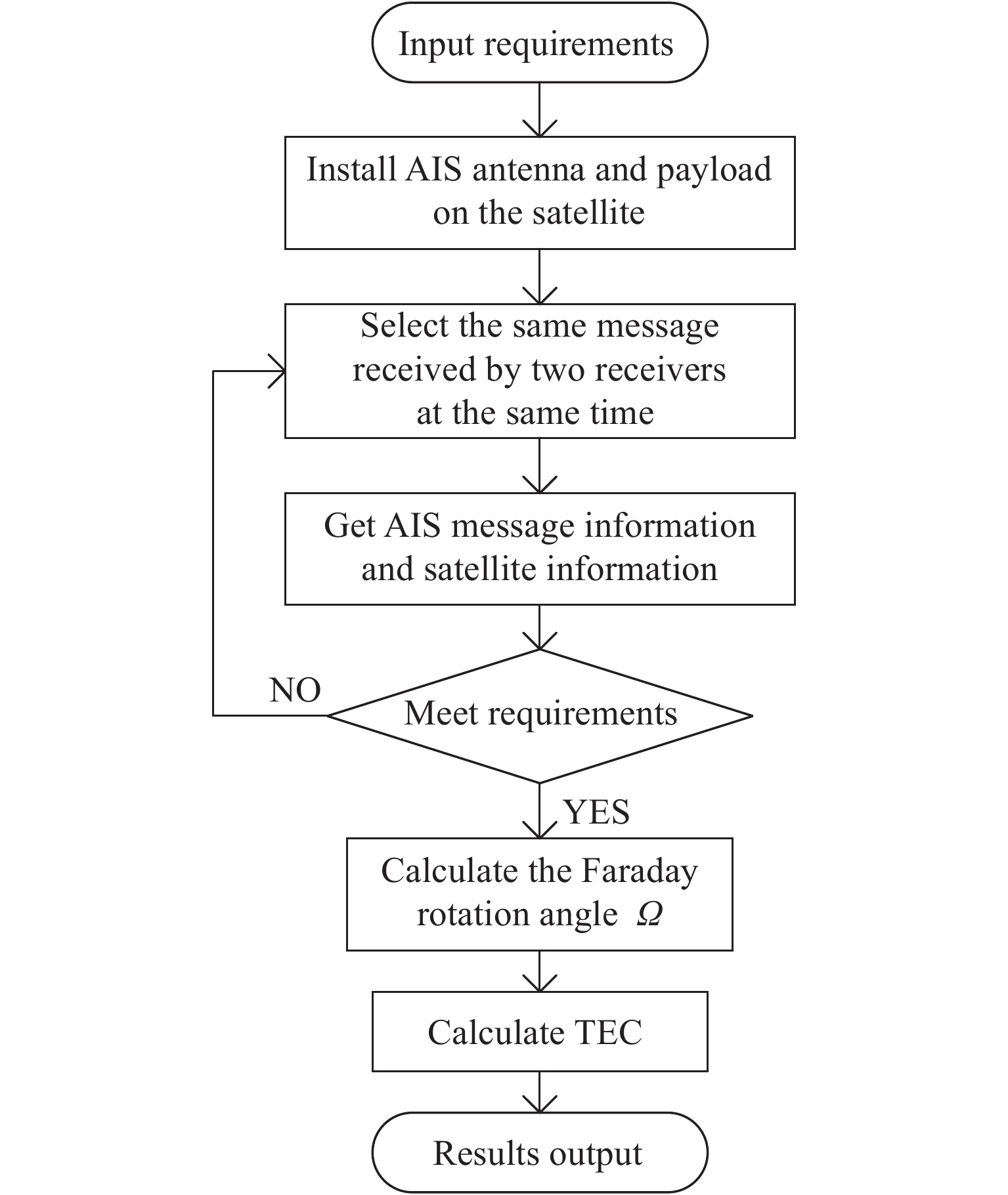
图 4 基于星载AIS数据的TEC测量方法流程
Figure 4. TEC measurement method based on space-based AIS data
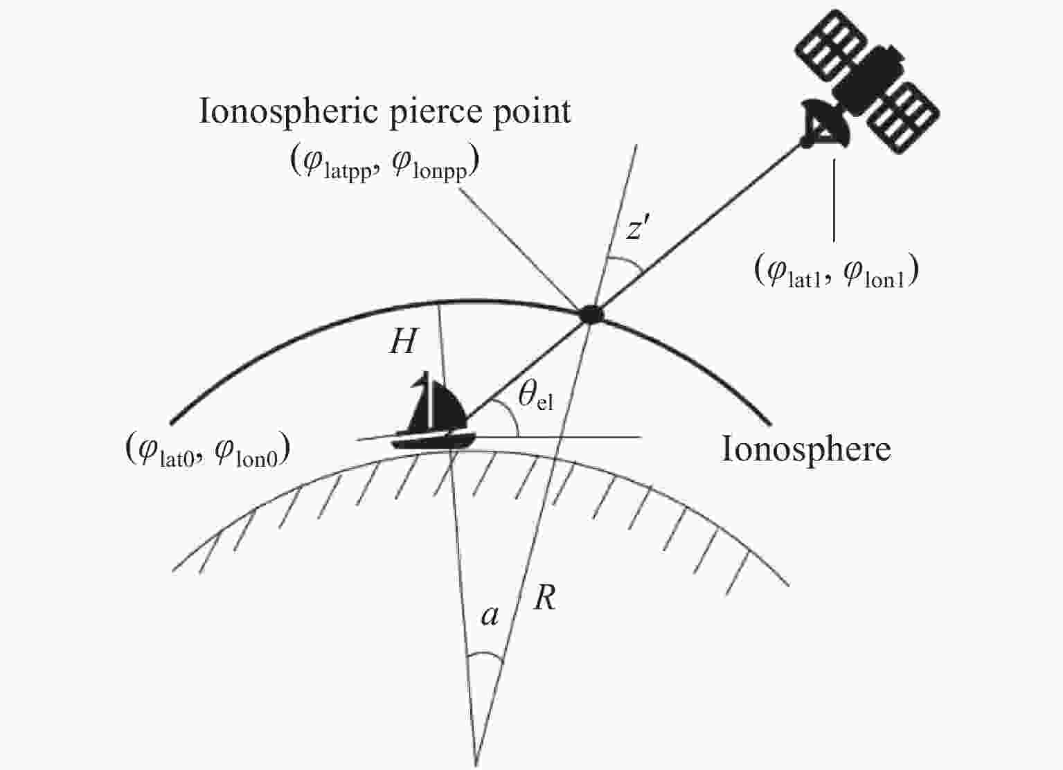
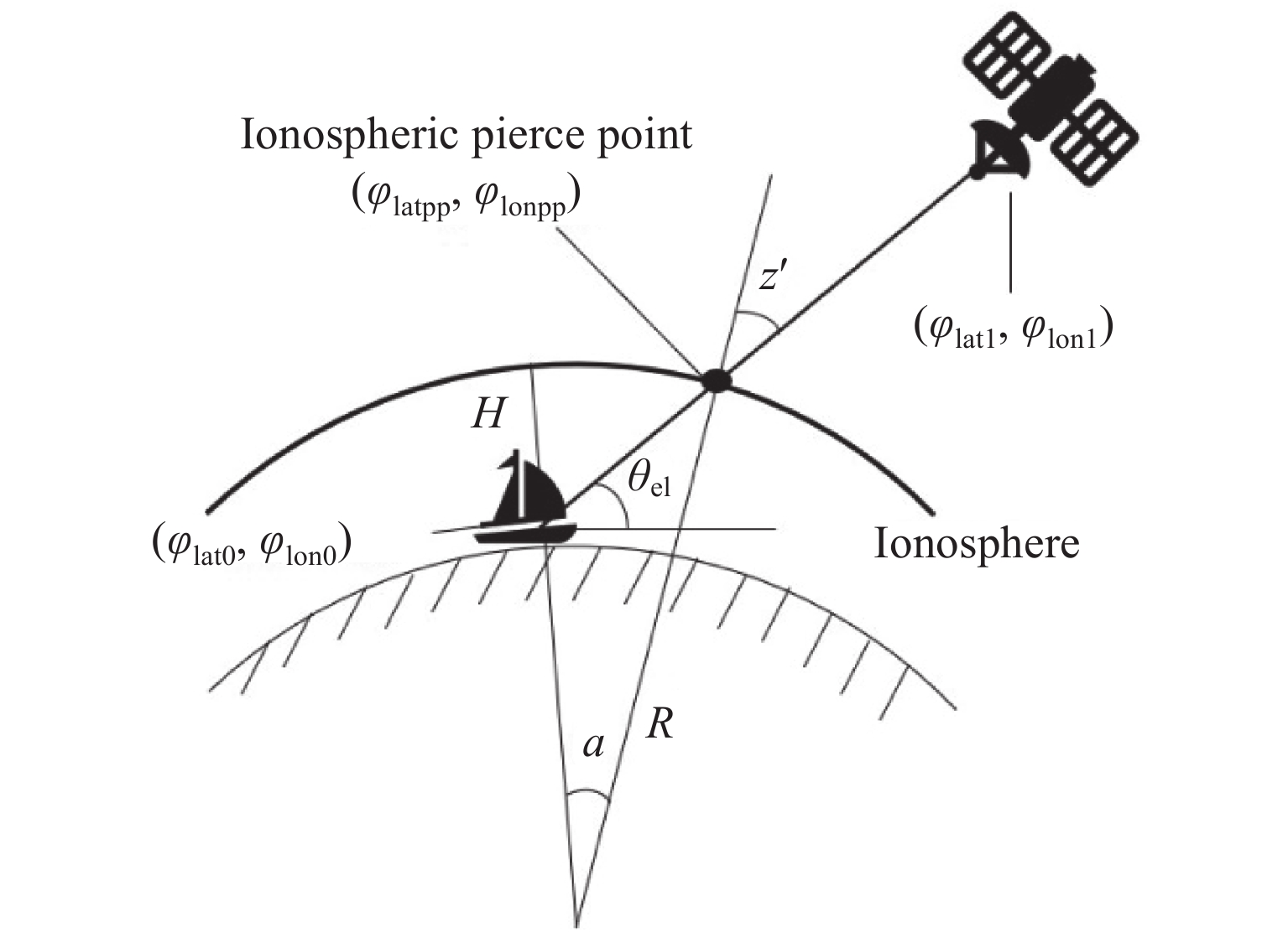
图 5 基于电离层薄层模型计算穿刺点
Figure 5. Calculating the puncture point based on the ionospheric single layer model
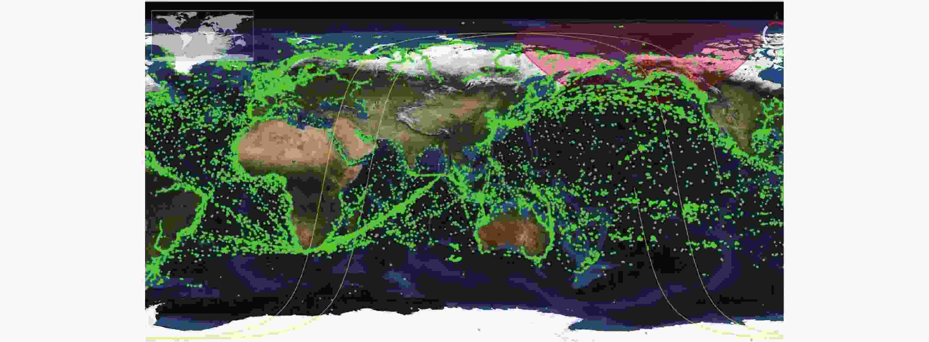
图 6 根据2020年8月23日天拓五号卫星接收到的AIS数据得到的船舶分布位置
Figure 6. Distribution of ships based on the AIS data received on the Tiantuo V satellite on 23 August 2020
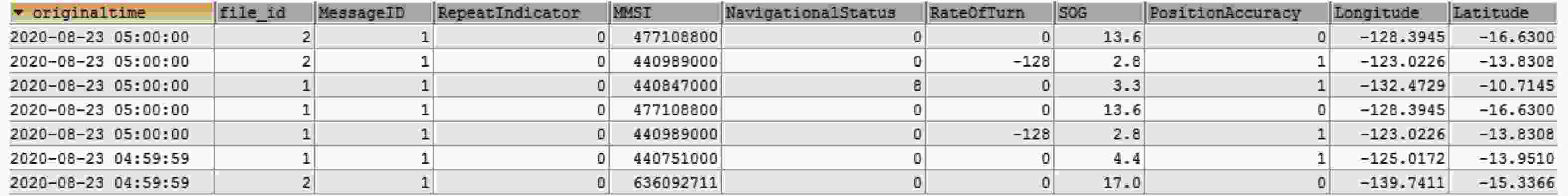
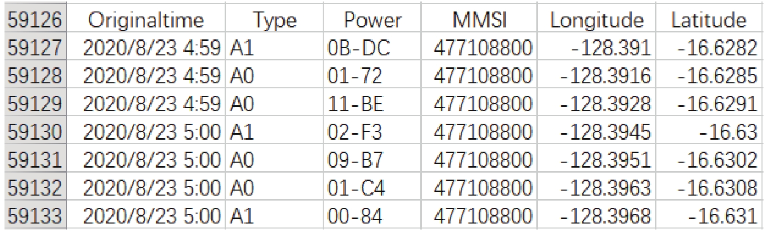
图 7 数据库中2020年8月23日天拓五号卫星两个接收机解码的AIS报文信息
Figure 7. AIS message information decoded by the two receivers of Tiantuo V satellite on 23 August 2020 in the database

图 8 2020年8月23日天拓五号A机解码的AIS报文信息
Figure 8. AIS message information decoded by A machine of Tiantuo V on 23 August 2020
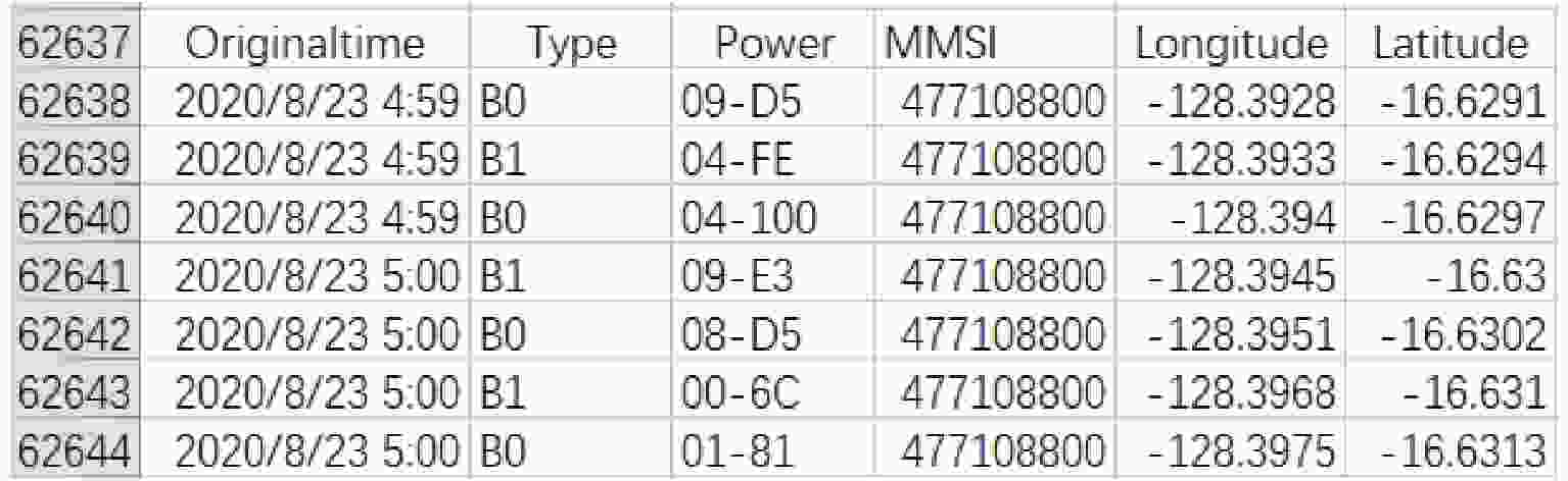
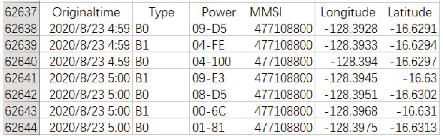
图 9 2020年8月23日天拓五号B机解码的AIS报文信息
Figure 9. AIS message information decoded by B machine of Tiantuo V on 23 August 2020
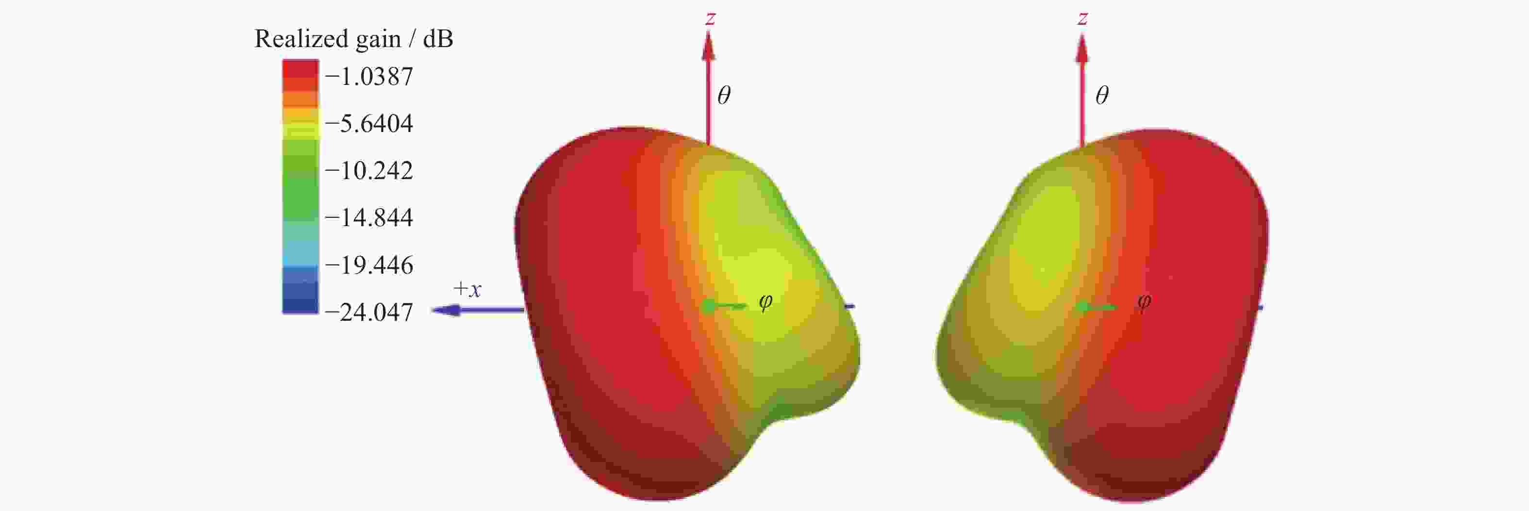
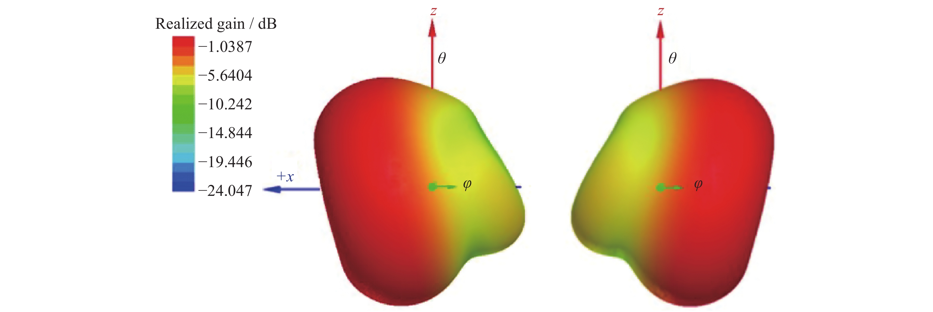
图 10 双AIS天线的全方向图(左边为AIS天线1方向图,右边为AIS天线2方向图)
Figure 10. Omni-directional pattern of dual AIS antennas (The left side of the figure is the pattern of AIS Antenna 1, and the right side is the pattern of AIS Antenna 2 )
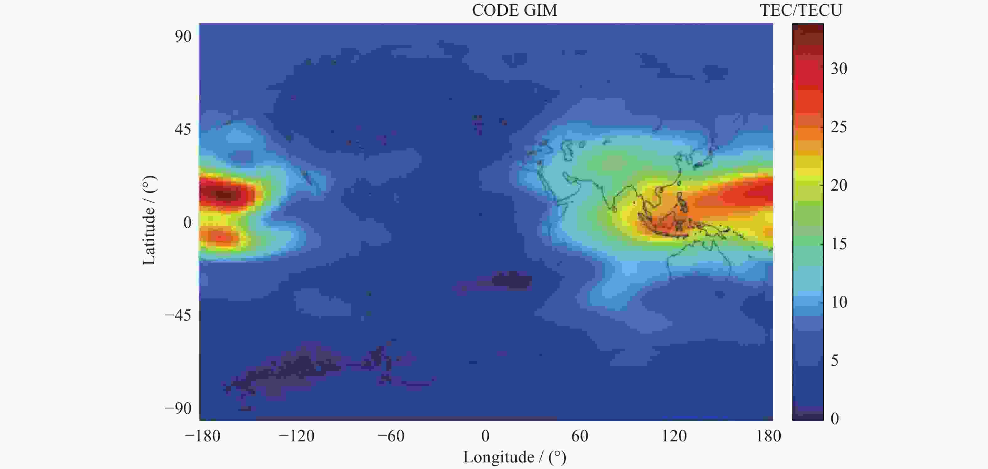
图 11 2020年8月23日05:00 UT的CODE的TEC分布
Figure 11. TEC distribution of CODE at 05:00 UT on 23 August 2020
表 1 本方法与CODE的TEC值对比
Table 1. Comparison of TEC value by this method and CODE
方法 时间(UT) 磁场强度/T 穿刺点位置坐标 法拉第旋转角/(°) TEC/TECU 本方法 05:00:00 $ 1.{\text{5535}} \times {10^{ - 5}} $ (15.73°S, 123.06°W) 73.7559 9.2052 CODE 05:00:00 - (15.73°S, 123.06°W) - 9.1083 本方法 05:00:03 $ 1.{\text{8379}} \times {10^{ - 5}} $ (15.76°S, 123.79°W) 84.5386 8.9128 CODE 05:00:03 - (15.76°S, 123.79°W) - 9.2120 本方法 05:00:08 $ 1.8{\text{408}} \times {10^{ - 5}} $ (15.50°S, 123.81°W) 99.4584 10.4760 CODE 05:00:08 - (15.50°S, 123.81°W) - 9.3140 本方法 04:59:58 $ 1.{\text{8168}} \times {10^{ - 5}} $ (15.97°S, 123.71°W) 83.1421 8.8674 CODE 04:59:58 - (15.97°S, 123.71°W) - 9.1265 本方法 04:59:55 $ 1.{\text{8422}} \times {10^{ - 5}} $ (15.91°S, 123.77°W) 87.9944 9.2616 CODE 04:59:55 - (15.91°S, 123.77°W) - 9.1937 本方法 06:00:04 $ -{\text{ 3}}{\text{.3630}} \times {10^{ - 5}} $ (30.76°S, 31.63°E) 84.4790 4.8706 CODE 06:00:04 - (30.76°S, 31.63°E) - 4.8267 本方法 05:59:59 $- {\text{ 3}}{\text{.2258}} \times {10^{ - 5}} $ (30.54°S, 31.67°E) 84.1913 5.0604 CODE 05:59:59 - (30.54°S, 31.67°E) - 4.8901 本方法 06:00:01 $ -{\text{ 4}}{\text{.4421}} \times {10^{ - 5}} $ (30.58°S, 34.98°E) 109.2740 4.7696 CODE 06:00:01 - (30.58°S, 34.98°E) - 5.3581 本方法 06:00:00 $ -{\text{ 4}}{\text{.5150}} \times {10^{ - 5}} $ (31.85°S, 34.68°E) 99.8255 4.2841 CODE 06:00:00 - (31.85°S, 34.68°E) - 5.0065 本方法 05:54:16 $ {\text{1}}{\text{.5267}} \times {10^{ - 5}} $ (10.82°S, 45.16°E) 87.7469 11.1440 CODE 05:54:16 - (10.82°S, 45.16°E) - 11.7851 本方法 05:53:39 $ {\text{1}}{\text{.6164}} \times {10^{ - 5}} $ (8.84°S, 45.33°E) 90.7516 10.8190 CODE 05:53:39 - (8.84°S, 45.33°E) - 12.2485 本方法 05:52:44 $ {\text{1}}{\text{.2077}} \times {10^{ - 5}} $ (5.39°S, 44.53°E) 90.4933 14.5290 CODE 05:52:44 - (5.39°S, 44.53°E) - 12.7368 本方法 05:52:32 $ {\text{1}}{\text{.6347}} \times {10^{ - 5}} $ (4.36°S, 45.21°E) 98.7884 11.7170 CODE 05:52:32 - (4.36°S, 45.21°E) - 12.9979 本方法 05:51:55 $ {\text{1}}{\text{.7622}} \times {10^{ - 5}} $ (1.99°S, 45.50°E) 115.5008 12.7080 CODE 05:51:55 - (1.99°S, 45.50°E) - 13.3356 本方法 05:32:02 $ {\text{2}}{\text{.5009}} \times {10^{ - 5}} $ (68.90°N, 58.05°E) 92.5313 7.1737 CODE 05:32:02 - (68.90°N, 58.05°E) - 7.4917 本方法 05:32:00 $ {\text{2}}{\text{.4395}} \times {10^{ - 5}} $ (67.54°N, 56.38°E) 108.8953 8.6543 CODE 05:32:00 - (67.54°N, 56.38°E) - 7.6025 本方法 05:31:56 $ {\text{2}}{\text{.5113}} \times {10^{ - 5}} $ (69.35°N, 59.29°E) 87.8939 6.7860 CODE 05:31:56 - (69.35°N, 59.29°E) - 7.4290 本方法 10:02:41 $ {\text{3}}{\text{.2143}} \times {10^{ - 5}} $ (54.66°N, 155.21°E) 110.3466 6.6562 CODE 10:02:41 - (54.66°N, 155.21°E) - 7.8275 本方法 10:02:58 $ {\text{3}}{\text{.6254}} \times {10^{ - 5}} $ (56.34°N, 152.97°E) 109.2740 6.3535 CODE 10:02:58 - (56.34°N, 152.97°E) - 7.7258 本方法 10:03:34 $ {\text{3}}{\text{.3470}} \times {10^{ - 5}} $ (58.46°N, 153.22°E) 103.8324 6.0112 CODE 10:03:34 - (58.46°N, 153.22°E) - 7.5037  下载: 导出CSV
-
[1] LIU Z Z. Ionosphere Tomographic Modeling and Applications Using Global Positioning System (GPS) Measurements[D]. Calgary: University of Calgary, 2004 [2] BERNHARDT P A, SIEFRING C L. New satellite-based systems for ionospheric tomography and scintillation region imaging[J]. Radio Science, 2006, 41(5): RS5S23 [3] KRANKOWSKI A, ZAKHARENKOVA I, KRYPIAK-GREGORCZYK A, et al. Ionospheric electron density observed by FORMOSAT-3/COSMIC over the European region and validated by ionosonde data[J]. Journal of Geodesy, 2011, 85(12): 949-964 doi: 10.1007/s00190-011-0481-z [4] LEI J H, SYNDERGAARD S, BURNS A G, et al. Comparison of COSMIC ionospheric measurements with ground‐based observations and model predictions: preliminary results[J]. Journal of Geophysical Research: Space Physics, 2007, 112(A7): A07308 doi: 10.1029/2006JA012240 [5] 訾海峰, 门志荣, 陈筠力, 等. 针对星载SAR法拉第旋转估计的NeQuick-2模型精度分析[J]. 上海航天, 2020, 37(5): 79-85ZI Haifeng, MEN Zhirong, CHEN Junli, et al. Accuracy evaluation of NeQuick-2 model for faraday rotation estimation of space-borne SAR[J]. Aerospace Shanghai, 2020, 37(5): 79-85 [6] 赵智博, 任晓东, 张小红, 等. 联合GNSS/LEO卫星观测数据的区域电离层建模与精度评估[J]. 武汉大学学报(信息科学版), 2021, 46(2): 262-269,295ZHAO Zhibo, REN Xiaodong, ZHANG Xiaohong, et al. Regional ionospheric modeling and accuracy assessment using GNSS/LEO satellites observations[J]. Geomatics and Information Science of Wuhan University, 2021, 46(2): 262-269,295 [7] TSAI L C, LIU C H, TSAI W H, et al. Tomographic imaging of the ionosphere using the GPS/MET and NNSS data[J]. Journal of Atmospheric and Solar-Terrestrial Physics, 2002, 64(18): 2003-2011 doi: 10.1016/S1364-6826(02)00218-3 [8] MEYER F, BAMLER R, JAKOWSKI N, et al. The potential of low-frequency SAR systems for mapping ionospheric TEC distributions[J]. IEEE Geoscience and Remote Sensing Letters, 2006, 3(4): 560-564 doi: 10.1109/LGRS.2006.882148 [9] JEHLE M, FREY O, SMALL D, et al. Measurement of ionospheric TEC in spaceborne SAR data[J]. IEEE Transactions on Geoscience and Remote Sensing, 2010, 48(6): 2460-2468 doi: 10.1109/TGRS.2010.2040621 [10] 赵海生, 许正文, 吴健, 等. 三频信标高精度TEC测量新方法[J]. 空间科学学报, 2011, 31(2): 201-207 doi: 10.11728/cjss2011.02.201ZHAO Haisheng, XU Zhengwen, WU Jian, et al. New hybrid method for high resolution TEC measurement with the tri-band beacon[J]. Chinese Journal of Space Science, 2011, 31(2): 201-207 doi: 10.11728/cjss2011.02.201 [11] CUSHLEY A C, NOËL J M. Ionospheric tomography using ADS-B signals[J]. Radio Science, 2014, 49(7): 549-563 doi: 10.1002/2013RS005354 [12] CUSHLEY A C. Ionospheric Tomography Using Faraday Rotation of Automatic Dependent Surveillance Broadcast (UHF) Signals: Ionospheric Measurement from ADS-B Signals[D]. Kingston: Royal Military College of Canada, 2016 [13] CUSHLEY A C, NOËL J M. Ionospheric sounding and tomography using automatic identification system (AIS) and other signals of opportunity[J]. Radio Science, 2020, 55(1): e2019RS006872 [14] VAN DER PRYT R, VINCENT R. A simulation of the reception of automatic dependent surveillance-broadcast signals in low earth orbit[J]. International Journal of Navigation and Observation, 2015, 2015: 567604 doi: 10.1155/2015/567604 [15] 刘宸, 刘长建, 鲍亚东, 等. 电离层薄层高度对电离层模型化的影响[J]. 空间科学学报, 2018, 38(1): 37-47 doi: 10.11728/cjss2018.01.037LIU Chen, LIU Changjian, BAO Yadong, et al. Effects of ionosphere shell height on ionospheric modeling[J]. Chinese Journal of Space Science, 2018, 38(1): 37-47 doi: 10.11728/cjss2018.01.037 [16] SMITH D A, ARAUJO-PRADERE E A, MINTER C, et al. A comprehensive evaluation of the errors inherent in the use of a two‐dimensional shell for modeling the ionosphere[J]. Radio Science, 2008, 43(6): RS6008 [17] WARDINSKI I, SATURNINO D, AMIT H, et al. Geomagnetic core field models and secular variation forecasts for the 13 th International Geomagnetic Reference Field (IGRF-13)[J]. Earth, Planets and Space, 2020, 72(1): 155 doi: 10.1186/s40623-020-01254-7 [18] FENG J D, HAN B M, ZHAO Z Z, et al. A new global total electron content empirical model[J]. Remote Sensing, 2019, 11(6): 706 doi: 10.3390/rs11060706 [19] JEE G, LEE H B, KIM Y H, et al. Assessment of GPS global ionosphere maps (GIM) by comparison between CODE GIM and TOPEX/Jason TEC data: ionospheric perspective[J]. Journal of Geophysical Research: Space Physics, 2010, 115(A10): A10319 doi: 10.1029/2010JA015432 [20] 李子申, 王宁波, 李敏, 等. 国际GNSS服务组织全球电离层TEC格网精度评估与分析[J]. 地球物理学报, 2017, 60(10): 3718-3729 doi: 10.6038/cjg20171003LI Zishen, WANG Ningbo, LI Min, et al. Evaluation and analysis of the global ionospheric TEC map in the frame of international GNSS services[J]. Chinese Journal of Geophysics, 2017, 60(10): 3718-3729 doi: 10.6038/cjg20171003 -
-

 下载:
下载:


计量
- 文章访问数: 1764
- HTML全文浏览量: 484
- PDF下载量: 47
-
被引次数:
0(来源:Crossref)
0(来源:其他)

